A while back, our director of embedded software approached us with an idea to build an edge AI demo on a touchscreen microcontroller. The user would draw something on the touchscreen with their finger, and a tiny neural network would attempt to recognize it, displaying its predictions.
Although standard MNIST (handwritten digits) would have been an option, we wanted to do something a bit more fun, and Google’s “Quick, Draw!” came to mind. This is a massive crowd-sourced dataset featuring 50 million doodles across 345 categories. While it originated as an online neural network guessing game, it serves as an excellent foundation for machine learning research—and, we would argue, a much more fun alternative to MNIST!

Here is how we built a standalone, deeply quantized sketch recognizer capable of running on a severely resource-constrained microcontroller. All project files and the complete co-design toolchain are open source. You can explore the code and deploy it yourself at https://github.com/maltanar/QuickDraw-brevitas.
The primary objective was to build an interactive edge AI sketch demonstration running locally on a touchscreen microcontroller devkit (specifically, an STM32H7B3I-DK). The workhorse here is an ARM Cortex-M7 with no neural network accelerators or similar hardware. Even though the hardware boasts several MB of total memory, we wanted to see how small we could get to make this a true TinyML project. We set the following technical goals:
Tiny footprint: Achieve a minimal memory footprint of ~1 KB for the neural network. We wanted it so small that you wouldn’t have to think twice about embedding it into your application. To achieve this, we knew we would likely have to resort to low-bit quantization.
Decent demo-able accuracy: Maintain 90%+ accuracy on a 10-class subset of the Quick, Draw! dataset. We settled somewhat randomly on a 10-class subset: smiley face, eye, tree, airplane, bicycle, apple, eyeglasses, book, cell phone, and car. These are everyday objects that are easy to sketch, making them highly relatable and practical for a live interactive demo.
Zero Dependencies: Generate a standalone C file with no external runtime, libraries, or interpreter. At the end of the day, a neural network is just a bunch of multiply-adds and some nonlinearity. There should be no need to drag a massive software stack into the project for such a small network. We also wanted the result to be easily integrated into a Zephyr project, which further motivated the dependency-free approach.
A Transparent, Hackable Open-Source Flow: Avoiding licensing fees is nice, but we also wanted true visibility. The goal was to build a transparent pipeline where we could see exactly what was happening under the hood at every stage. Instead of wrestling with massive, opaque codebases or relying on proprietary “black-box” software, we wanted a setup that was easy to inspect, understand, and manually tweak to squeeze the neural network down to a minimal size.
There are quite a few strong options out there for TinyML. However, when evaluating how to develop and deploy our sketch recognizer, existing frameworks and standard deep learning architectures did not quite match our technical goals.
Here is what the landscape looked like for tools and deployment on a Cortex-M7:
Next, we looked at how others have approached the “Quick, Draw!” dataset. There were a few examples that served as a good starting point, including some with open-source code on GitHub, but nothing checked all our requirements immediately:
CNN + LSTM Networks (El Mouna et al.): Combining spatial and temporal features achieves roughly 95% accuracy on a 10-class subset, but it requires about 200k parameters running at full 32-bit floating-point (fp32) precision.
QuickDraw-pytorch on GitHub (Junyi Cao): This repository offered the possibility of using standard ResNet architectures, but they are way too large—ResNet18 needs 11 million parameters! However, it also included a bare-bones, standard CNN implementation requiring around 33k fp32 parameters to hit 95% accuracy. This was much closer to our goal, so we picked this repo as our starting point.
However, 33k parameters stored in fp32 still require over 130 KB of storage, more than 100 times our target footprint. We would need to perform some architecture search and heavy quantization to get there.
To achieve a transparent development and deployment pipeline with a no runtime overhead, we pieced together a modular, open-source stack with control and complete visibility at every stage:
Developed by AMD Research, Brevitas is a highly flexible PyTorch library for neural network quantization. While Post-Training Quantization (PTQ) can be completed in minutes, it is often useless for extreme 4-bit or 1/2-bit compression. Brevitas allows us to leverage Quantization-Aware Training (QAT). By propagating gradients directly through the quantized graph during training, QAT minimizes accuracy loss and models how the neural network will perform under severe bitwidth constraints. Although Brevitas lacks a native deployment engine, it is possible to export the trained network to ONNX or QONNX (an extension of ONNX that can represent arbitrary-precision quantization) interchange formats.
To bridge the gap between training and microcontroller deployment, the next step was to export the quantized model to ONNX (Open Neural Network Exchange). Managed as an open-source project under the Linux Foundation, ONNX provides a serialized neural network graph layout based on Protobuf. It features a strictly versioned operator specification, and its extensive ecosystem of Python libraries makes it perfect for manual or automated graph manipulation. This allowed us to inspect the raw graph, verify how operators were serialized including the datatypes, and manipulate the topology when required to achieve a smaller footprint for the deployment.
For the final translation to the microcontroller, we used emmtrix-onnx-cgen from emmtrix Technologies. This open-source tool ingests the standardized ONNX graph and converts it directly into pure C code and static data arrays. While emmtrix offers a proprietary, closed-source optimizer, we relied strictly on their open-source compiler variant. Though the open-source version is not heavily optimized out of the box, this was not a major hurdle for our tiny neural network. More importantly, it fulfilled our core philosophy: it gave us absolute transparency over the generated source code, exposing every layer, loop, and array allocation for possibilities for manual optimization.
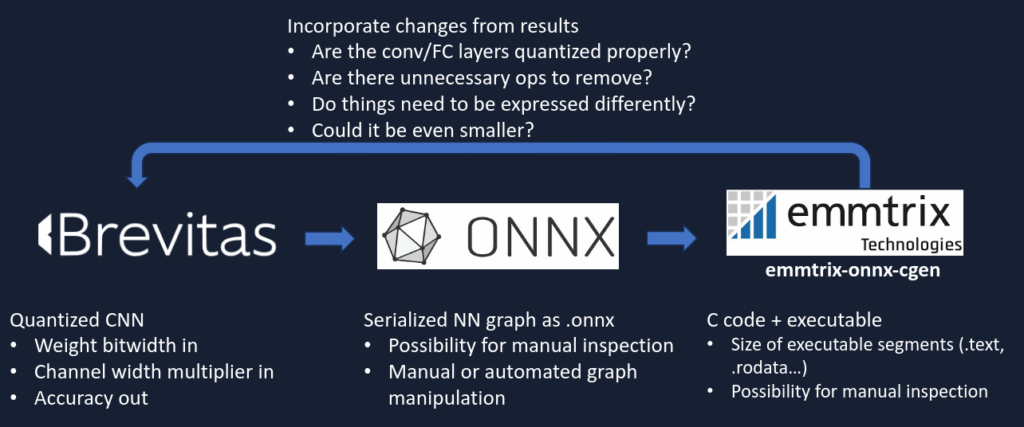
With a standalone C file as our output, we unlocked a highly “hackable” co-design loop. By manually inspecting the executable segments (.text, .rodata, etc.), we could identify inefficiencies and feedback changes directly to our network design, as shown in the illustration below.
Now it was time to do some neural architecture search and quantization exploration: we ran a hyperparameter sweep on the base CNN with added weight- and activation quantization. The Cortex-M7 supports down to 8-bit arithmetic, although it is possible to apply bit packing techniques to further shrink the memory footprint for weights. Thus, we opted to fix activations at 8-bits, while allowing weight quantization to go down to as low as a single bit per weight. For each point we explore, we used the total number of parameter bits as the cost metric to perform our cost-benefit analysis. You can see the results of the exploration below.
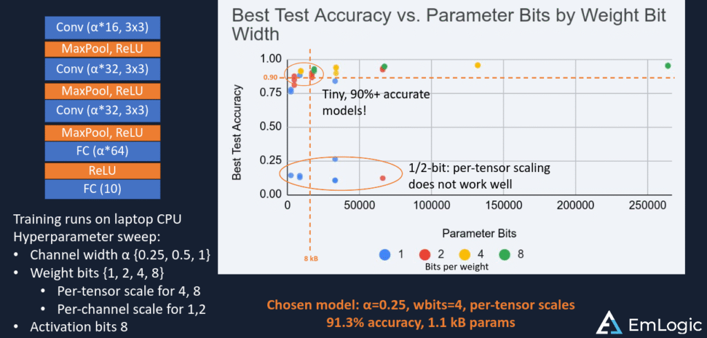
Ultimately, we settled on a configuration using a channel width multiplier of 0.25, 4-bit weights, and per-tensor scales. This model hit the exact sweet spot we needed: achieving 91.3% test accuracy with a parameter footprint of just 1.1 kB.
We can use Netron to examine the exported ONNX graph, which is very useful for understanding how the quantization and operators look like:
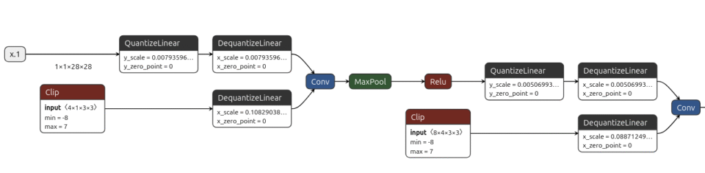
Quantization is the process of mapping real-valued numbers to a small integer range so models run faster and lighter on real hardware. In practice, a float value x is mapped to an integer q using a scale s and zero-point z, then mapped back with dequantization when needed. Quantize means “pack the value into integer form.” Dequantize means “reconstruct an approximate real value from that integer.” The approximation comes from rounding and clipping. So-called fake quantization in neural network deployment is when a model simulates that integer behavior but still executes much of the graph in floating point. You still see quantize and dequantize nodes, but the main compute path often remains float Conv and MatMul. This is useful during training and export because it helps preserve numerical behavior but it does not always match how we want deployment kernels to actually run. When we run this model through emmx-onnx-cgen:
// our weight tensors are in int8_t - not int4 but still...yay?
extern const int8_t weight4__layer1_layer1_0_weight_quant_export_handler_constant_1_output_0[4][1][3][3];
const EMX_UNUSED int8_t weight4__layer1_layer1_0_weight_quant_export_handler_constant_1_output_0[4][1][3][3] = {
    {
        {
            {
                -8, -8, -3
            },
// ...

// but our conv kernel compute is in fp32 - boo!
EMX_NODE_FN void node4__layer1_layer1_0_conv(const float input0[1][1][28][28], const float weights[4][1][3][3], float output[1][4][28][28]) { // ...
We can see that our weights are in int8 arrays – although there is a BitInt type in the C23 standard, this still uses 8-bit datatypes under the hood. Since we have access to the C code and can manipulate it as we want, we could switch over to using libraries like libbitpack to save half the parameter space, although for this demo it doesn’t matter too much since the footprint is already tiny. A larger concern is the computation of the MAC-heavy convolution kernel being executed as floating point computation – why is that happening? It’s because of the “fake quantization” representation discussed above.
Luckily, it is not hard to see how the integer operations can be separated from the floating point scale factors – as long as the scales are per-tensor (or possibly per-channel for weights) we can first do the MAC-heavy computation with integers, and then apply the scale factor afterwards. There’s quite a bit of a rabbit hole here which we won’t dive into, but here is further reading if you are interested. For this demo, we put together a script in Python which converts the QuantizeLinear -> Conv/MatMul -> DequantizeLinear chains in the graph into integer-friendly forms such as QLinearConv, QLinearMatMul, ConvInteger, MatMulInteger when possible. Inspecting the converted graph in ONNX and the generated C code, we can see that the computationally heavy operations have been successfully converted to int8.
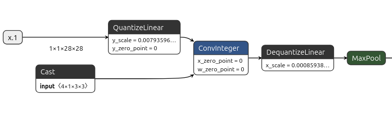
// conv computation is now in int8!
EMX_NODE_FN void node2_conv_0_integer(const int8_t input0[1][1][28][28], const int8_t weights[16][1][3][3], const int8_t x_zero_point[1], int32_t output[1][16][28][28]) { //..
There are numerous other optimizations we could apply to the C code, including but not limited to:
Remove unused zero-point computation logic and variables
Fuse ReLU into previous layer for fewer function calls and variables
Staged instead of global tensor allocations
Optimize convolutional kernels with DSP instructions
Bit-packing on weights to further shrink the footprint
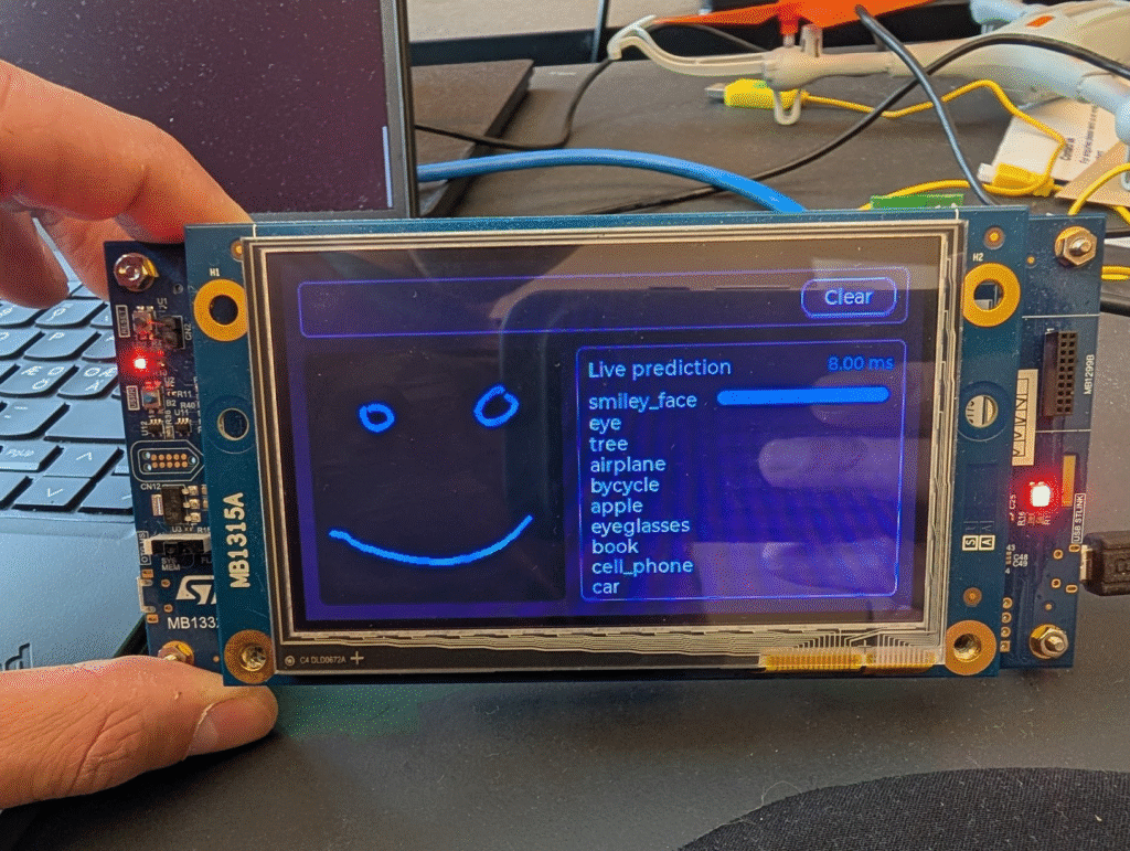
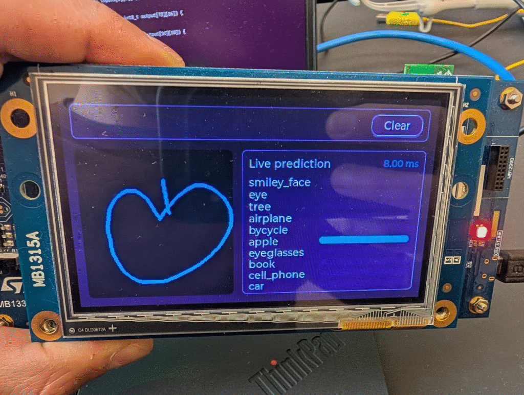
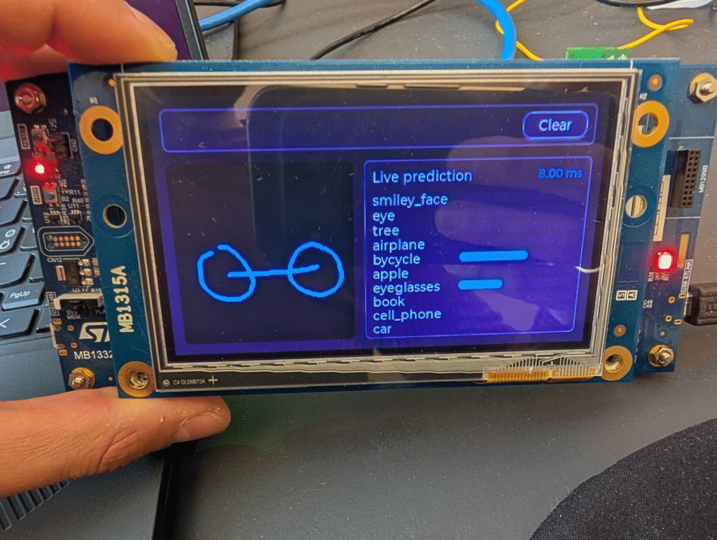
Now that we have a standalone C implementation of our sketch recognition neural network, it was time to build a demo. Based on this previous blog post on graphics frameworks, we opted for Zephyr + LVGL as the environment, which made it a breeze to quickly bootstrap a GUI with sketching, display of the inference results and an inference runtime indicator. The user draws freehand sketches on the board’s touchscreen display. On each pen-up event, the drawing is downsampled to a 28×28 grayscale image and fed into the trained neural network that classifies the sketch into one of 10 categories: smiley face, eye, tree, airplane, bicycle, apple, eyeglasses, book, cell phone, or car. A live bar chart shows the softmax probability for each class, updating instantly after every stroke.
You can see the demo in action below on three different sketches, showing an inference time of 8 ms.
Yaman Umuroglu is a Principal Edge AI Designer at EmLogic, where he specializes in deploying highly efficient, specialized machine learning models on FPGAs, microcontrollers, and other resource-constrained devices. He was previously a Principal Engineer at AMD/Xilinx Research working on neural network-hardware co-design for Edge AI on FPGAs.
Ivan Pfarher is an Experienced Senior Embedded Software Developer (10+ years) specializing in low-level firmware, device drivers, and hardware-adjacent software for MCUs, MPUs, SoCs, and SoMs at EmLogic. He is skilled in board bring-up, hardware debugging, and system troubleshooting. His industry background spans embedded Linux, satellite/aerospace, industrial automation, and consumer products.