Earth observation satellites (or Eyes in the Sky, as you could think of them) are useful for a surprising number of things: detecting wildfires and assessing damage after natural disasters, spotting dark vessels that switch off their transponders, finding routes through sea ice, monitoring crops and forests, and so on. The basic recipe is always the same – take pictures of the Earth’s surface, beam them down to the ground, and let big computers crunch through them.

So, the Eye in the Sky has a wireless optic nerve running down to Earth, and that last bit is often the problem. A satellite in Low Earth Orbit (LEO) can only talk to a ground station while it’s above the horizon, which typically means a pass of around 10 minutes, a handful of times per day. Even a large flagship mission like Landsat 8 has an X-band downlink of a few hundred Mbps, and a CubeSat with an S-band radio gets a tiny fraction of that. Meanwhile the cameras could keep producing data whether or not there is a ground station in sight, so prioritization is rather important.
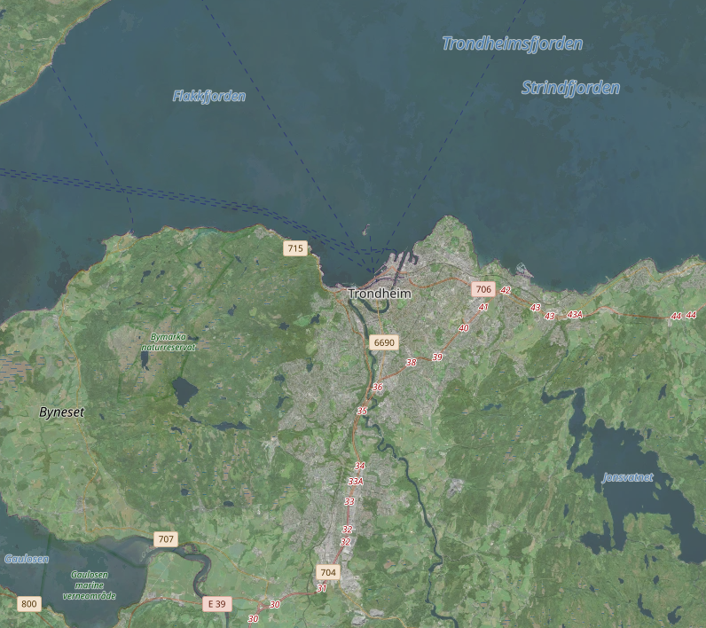
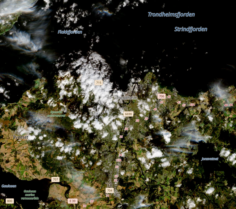
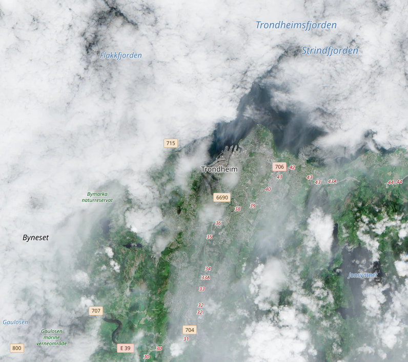
Three satellite views of Trondheim, including on a rare clear day to the left. Contains modified Copernicus Sentinel data 2026 for Sentinel data processed in Copernicus Browser.
To make it worse: clouds. Several studies estimate that around 67% of the Earth’s surface is covered by clouds at any given time, and it doesn’t get better at high latitudes – satellite-based estimates put the annual mean cloud cover over the Arctic at up to 78%. As someone writing this from Trondheim in November, I can confirm this from personal experience. Unless you are flying a (relatively expensive) Synthetic Aperture Radar (SAR) that sees through clouds, an optical satellite would spend a large part of its life taking very high resolution pictures of the tops of clouds, and then dutifully queue them up for the downlink.
The obvious fix is to look at each image in orbit, figure out whether it’s mostly cloud, and act accordingly – drop it, deprioritize it, or compress it harder, while the clear images go to the front of the queue. This isn’t a new idea: ESA’s Φ-lab famously flew it on the Φsat-1 mission with CloudScout, a convolutional neural network (CNN) running on an Intel Myriad 2 VPU that classified hyperspectral images as cloudy or not, reaching 92% accuracy with a 1% false positive rate.
Note the wording false positive there, since it’ll come up several more times in this post. Here, a positive means “this tile is cloudy”, so a false positive means we label a perfectly good, clear image as cloudy and potentially throw it away. That’s the expensive mistake: sending down the occasional cloudy image just wastes some bandwidth, but discarding the one clear image of the wildfire you were looking for is much worse. So we care about both accuracy and the False Positive Rate (FPR).
If we want a neural network on a satellite, do we just put a desktop GPU in a metal box and launch it? That doesn’t quite cut it, as it turns out:
Power and Thermal: A small CubeSat typically has a power budget of a few to a few tens of watts in total, shared between the radio, control, the payload and everything else. What’s more – space is cold, but it’s surprisingly hard to cool electronics there. There is no air for convection, so heat can only leave through conduction to the structure and radiation off its surfaces. Every watt we burn needs a path out, so ideally we should be burning as few watts as possible.
Throughput: If we want to run our camera all the time, the classifier must keep up with a moving target – literally! A LEO satellite’s ground track moves at roughly 7 km/s, and the camera keeps sweeping out new image lines the whole time. Depending on the resolution and swath width, that adds up to anywhere from millions of pixels per second for a medium-resolution imager like Landsat 8’s up to around a billion pixels per second for the sharpest commercial ones.
Reliability: Radiation causes Single Event Upsets (SEUs) that flip bits in memories and registers, and depending on the orbit and mission lifetime this ranges from an occasional nuisance to a design-defining constraint. Fewer external components (like DRAM) and simpler data paths make mitigation easier.
Luckily, FPGAs tick a lot of those boxes, and they are already on board most satellites for tasks like payload data handling, image compression and communications. Radiation-tolerant FPGAs are an established product category, and even off-the-shelf commercial parts like the Zynq-7000 series fly on many CubeSats with mitigation techniques such as configuration memory scrubbing. A great example close to home is NTNU’s HYPSO hyperspectral imaging satellites, which use a Zynq-7000 SoC to process their hyperspectral data cubes on board. So in many cases, we don’t even need to add a new chip to the satellite – we can just add a new circuit to an FPGA that’s already there.
How do we put a neural network on an FPGA? One option is a programmable overlay like the AMD/Xilinx DPU, which is essentially a programmable neural network accelerator implemented on the FPGA that runs instructions compiled from your network. That works, but it’s a one-size-fits-all design with a fixed precision (int8), it needs external DRAM for weights and activations, and it takes a sizable chunk of the FPGA. We can do much better by customizing the hardware and the neural network together. This is exactly what FINN does (which yours truly helped create at Xilinx Research back in the day). FINN takes a quantized neural network and generates a dataflow accelerator, where each layer becomes its own hardware block with its weights in on-chip memory, all connected by FIFOs, and the parallelism of each layer can be tuned to hit a target throughput. No instruction stream, no external memory for the accelerator, and only as much hardware as the network actually needs. For this project, we used FINN with some extra EmLogic optimizations on top. Now let’s see what this technology can do for cloud screening.
Rather than inventing everything from scratch, I decided to base the demo on CloudSatNet-1 by Pitonak et al. from Zaitra: a quantized CNN trained with Brevitas and deployed with FINN on a Zynq-7020 – the same chip as on the PYNQ-Z1 I will be using, which makes for a nice apples-to-apples comparison. Their network classifies 512×512 RGB tiles from the Landsat 8 Cloud Cover Assessment Validation dataset (also known as the L8 Biome dataset) as cloudy or clear, using 10 convolutional and 2 fully connected layers. Their reported FPGA results look like this:
| Bit width | Acc. (SI incl.) % | Acc. (SI excl.) % | FPR (SI excl.) % | FPS | LUTs (of 53,200) | FFs | BRAM36 (of 140) | DSP | Avg. power (W) |
|---|---|---|---|---|---|---|---|---|---|
| 4-bit | 87.42 | 94.84 | 5.72 | 15.47 | 36,735 (69%) | 51,721 | 88 | 30 | 2.59 |
| 3-bit | 88.24 | 93.37 | 4.17 | 15.47 | 31,335 (59%) | 42,975 | 67 | 30 | 2.56 |
| 2-bit | 83.41 | 92.08 | 5.14 | 15.46 | 25,387 (48%) | 34,569 | 46 | 30 | 2.52 |
What is “SI”? The L8 Biome dataset has 96 scenes across 8 biomes, one of which is Snow/Ice – and it’s arguably the most interesting one. Simpler cloud detectors that threshold pixel brightness tend to fail spectacularly here, since clouds and snow are both bright and white, so a snowy mountain range gets flagged as one big cloud. A neural network can do better by picking up on texture, shape and context rather than just color: for instance, snowfields have sharp edges and follow the terrain, while clouds are fluffy and cast shadows. Still, with only RGB to go on, even a neural network gets fooled sometimes – a thin veil of cloud over a glacier is genuinely hard to call, and the false positive rate suffers. The paper therefore reports results both including and excluding the Snow/Ice biome, and the headline numbers are for the latter.
A few things stood out to me here. All three variants are stuck at ~15.5 frames (tiles) per second regardless of bit width, and the authors point out that the first layer is the bottleneck. 69% of the LUTs on a Zynq-7020 also doesn’t leave a lot of room for much else on the FPGA. So I wanted to see if we could improve upon this design.
To keep the comparison fair, we stuck to the paper’s dataset preparation and overall network structure: 512×512 RGB tiles from the L8 Biome dataset, labeled cloudy when at least 70% of the tile is covered by cloud according to the dataset’s masks. The network is trained with quantization-aware training in Brevitas, with 4-bit weights and activations in the hidden layers and 8 bits for the first and last layers. It’s pleasantly tiny at 18,424 parameters, or ~16 KB of weights, although it still needs 152 million multiply-accumulates per tile. The accelerator is generated with FINN, with some extra EmLogic optimizations on top that squeeze more out of the same chip.
Here’s how we compare to the CloudSatNet-1 4-bit model on the same Zynq-7020 chip:
| CloudSatNet-1 (4-bit) | Ours (4-bit) | |
|---|---|---|
| Accuracy / FPR (SI excl.) | 94.84% / 5.72% | 93.54% / 4.32% |
| Throughput | 15.47 tiles/s | 33.89 tiles/s |
| LUTs | 36,735 (69%) | 18,186 (34%) system, 11,343 (21%) accelerator |
| FFs | 51,721 (49%) | 17,732 (17%) system, 8,552 (8%) accelerator |
| BRAM36 | 88 (63%) | 57.5 (41%) system, 55.5 (40%) accelerator |
| DSP | 30 | 32 |
| Power | 2.59 W | 2.36 W (board total) |
Accuracy: We land about 1 percentage point behind the paper on accuracy, but with a lower false positive rate – which, as we discussed, is the more expensive mistake. It should be said that clouds and snow remain hard to tell apart in pure RGB, however: with the Snow/Ice biome thrown back in, the FPR jumps to 17%.
Performance: On a PYNQ-Z1 with the accelerator clocked at 100 MHz, we measured 33.89 tiles/s, which is 26.6 MB/s of RGB imagery, with a latency of 31 ms per tile. That’s 2.2x the throughput of the paper, or ~8.9 million pixels per second – comfortably in the range of a medium-resolution imager.
FPGA resources: The accelerator itself uses 11.3k LUTs, 32 DSPs and the equivalent of ~56 BRAM36 – without any external memory. Even with the DMA engines and interconnect added, the whole design fits in about a third of the Zynq-7020’s LUTs, leaving the rest of the FPGA free for other payload tasks. If we wanted more throughput, we could easily scale up the FINN-generated accelerator, though as you’ll read a bit later, the performance in our demo is currently bottlenecked by reading images from the SD card.
Power: I measured the board’s power draw with a USB power meter. With the FPGA unconfigured and Linux idling on the ARM cores, the PYNQ-Z1 draws 1.64 W. With the bitstream loaded and the accelerator idle, it’s 1.74 W, and while running the full demo it’s 2.36 W total. Note that the 2.36 W is the entire board, including the ARM cores feeding tiles to the accelerator, DDR, Ethernet and the various regulators – a dedicated payload board would do noticeably better.
As I unfortunately don’t have any satellites lying around on my desk, we’ll have to make do with a dashboard for this demo. It currently goes through nine scenes from the L8 Biome dataset, cuts them into tiles, and streams them through the accelerator while painting the result on top of the scene: tiles the FPGA would drop turn into cloud, the rest are kept for downlink. Live counters show throughput, accuracy against the ground truth masks, and how much downlink we’ve saved. You can see the demo in action in the video above.
The PyQt dashboard in the demo runs entirely on the board, driving an HDMI display straight from the FPGA using a custom fork of pynqz1fb. In this setup it’s actually the little ARM cores reading tiles off the SD card that set the pace at ~15 tiles/s, not the accelerator. In a real deployment, the image stream would not be coming directly from a low-bandwidth SD card read, and we could potentially scale up the accelerator to much higher throughput by taking up more FPGA resources.
On-board cloud screening is a great example of why AI at the edge matters: the cheapest byte to downlink is the one you never send. By co-designing a 4-bit quantized CNN with a FINN-generated dataflow accelerator and our own optimizations on top, we got 93.5% accuracy at 4.3% FPR, 34 tiles/s in 2.36 W of total board power, using only 21% of the LUTs on a Zynq-7020 and no external memory – more than doubling the throughput of the published baseline while using half the LUTs for the complete system. Building on open-source foundations like Brevitas and FINN also means no black-box toolchain or vendor lock-in standing between the neural network and the hardware.
At EmLogic, we offer Edge AI design services across platforms and applications, with special expertise in FPGA acceleration and space systems. Whether you need a sparring partner for an early idea or a turnkey solution, if you want to see what is possible for your (Space-)Edge AI applications, please feel free to reach out!
Yaman Umuroglu is a Principal Edge AI Designer at EmLogic, where he specializes in deploying highly efficient, specialized machine learning models on FPGAs, microcontrollers, and other resource-constrained devices. He was previously a Principal Engineer at AMD/Xilinx Research working on neural network-hardware co-design for Edge AI on FPGAs.